Track your first experiment

This page reuses the quick-start project and working directory from Create a project. Complete that page before continuing.

Run two training simulations on your machine, compare them, then schedule the same simulator with the Polyaxon Agent (compute cluster). All three runs send their parameters, metrics, and visualizations to the same project.

Run the simulator locally

Download the example:

curl -fLO https://raw.githubusercontent.com/polyaxon/polyaxon-quick-start/master/tracking/simulate_dl_experiment.py

Run a baseline experiment:

python3 simulate_dl_experiment.py \
  --project=quick-start \
  --run-name=baseline \
  --epochs=20 \
  --seed=42 \
  --batch-size=64 \
  --learning-rate=0.001

The script simulates 20 training epochs with a fixed seed. It does not train a model or need a GPU, but its loss and accuracy respond to the supplied hyperparameters. It logs:

• Hyperparameters as run inputs.
• Training, validation, and per-class metrics at each epoch.
• Weight and gradient histograms at regular checkpoints.
• Confusion matrices and ROC and precision-recall curves.
• Weight distributions, gradient flow, feature activations, and loss-landscape images.
• Progress, text snapshots, and final and best results.

The full simulator logs all the event types listed above. Its basic tracking lifecycle is:

from polyaxon import tracking

tracking.init(project="quick-start", name="baseline", tags=["sim"])
tracking.log_inputs(learning_rate=0.001, epochs=20)

for epoch in range(20):
    tracking.log_metrics(
        step=epoch,
        train_loss=0.5,
        val_accuracy=0.8,
    )

tracking.log_outputs(best_val_accuracy=0.8)
tracking.end()

The downloaded script expands this loop with per-class metrics, histograms, curves, images, progress, and text events.

When the run finishes, the script prints its Polyaxon run UUID.

Inspect the run

Open the project dashboard:

polyaxon project dashboard --project=quick-start --yes

Open the run named baseline. Its inputs and outputs describe the experiment, while its metrics and visualizations show how training changed across epochs.

polyaxon ops ls -p quick-start

export RUN_UUID=PASTE_BASELINE_RUN_UUID_HERE
polyaxon ops dashboard -p quick-start -uid $RUN_UUID --yes

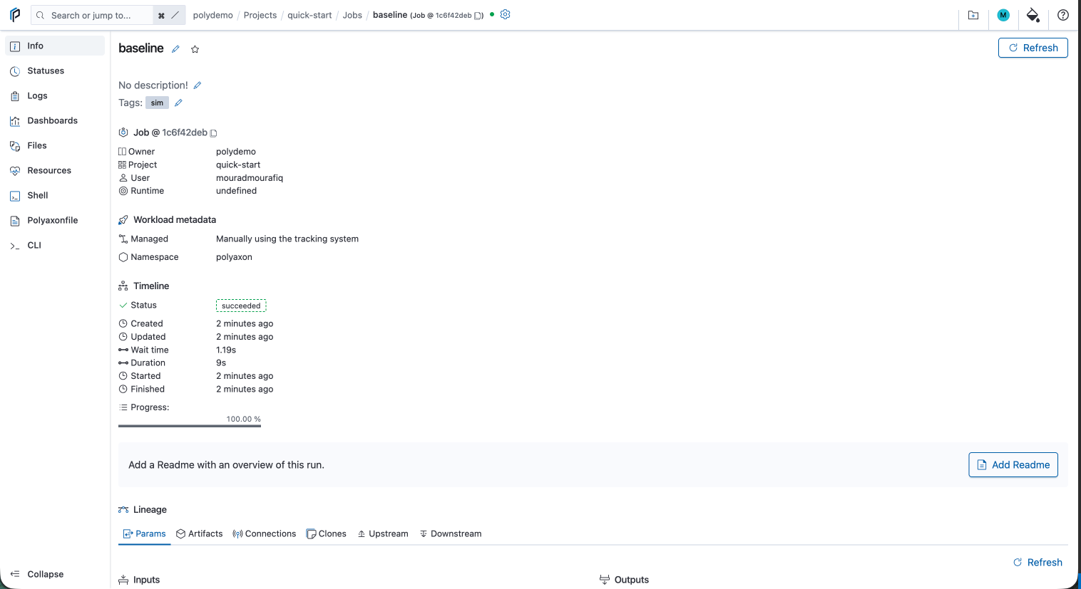
The Info view shows the run's identity, status, and execution metadata. Your run UUID and timestamps will differ from this example.

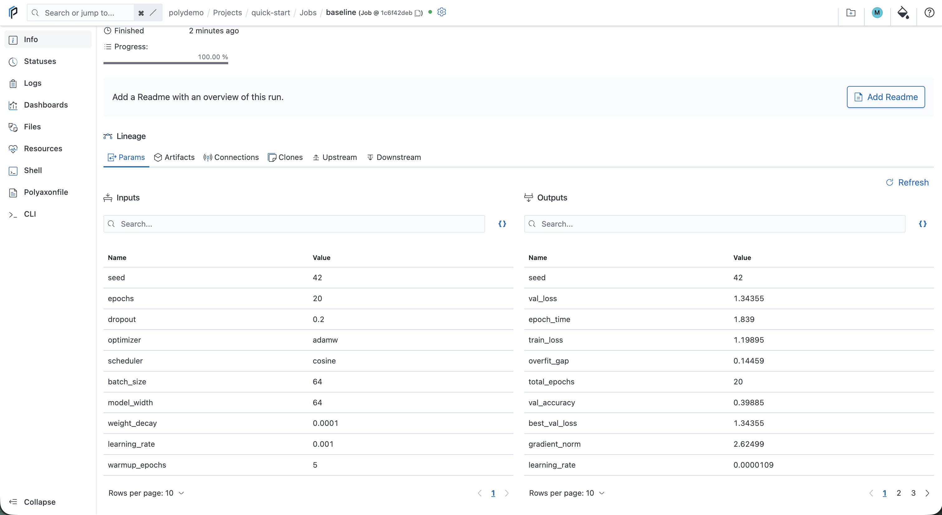
The Lineage section lists the inputs recorded before the simulation and the outputs logged when it finished.

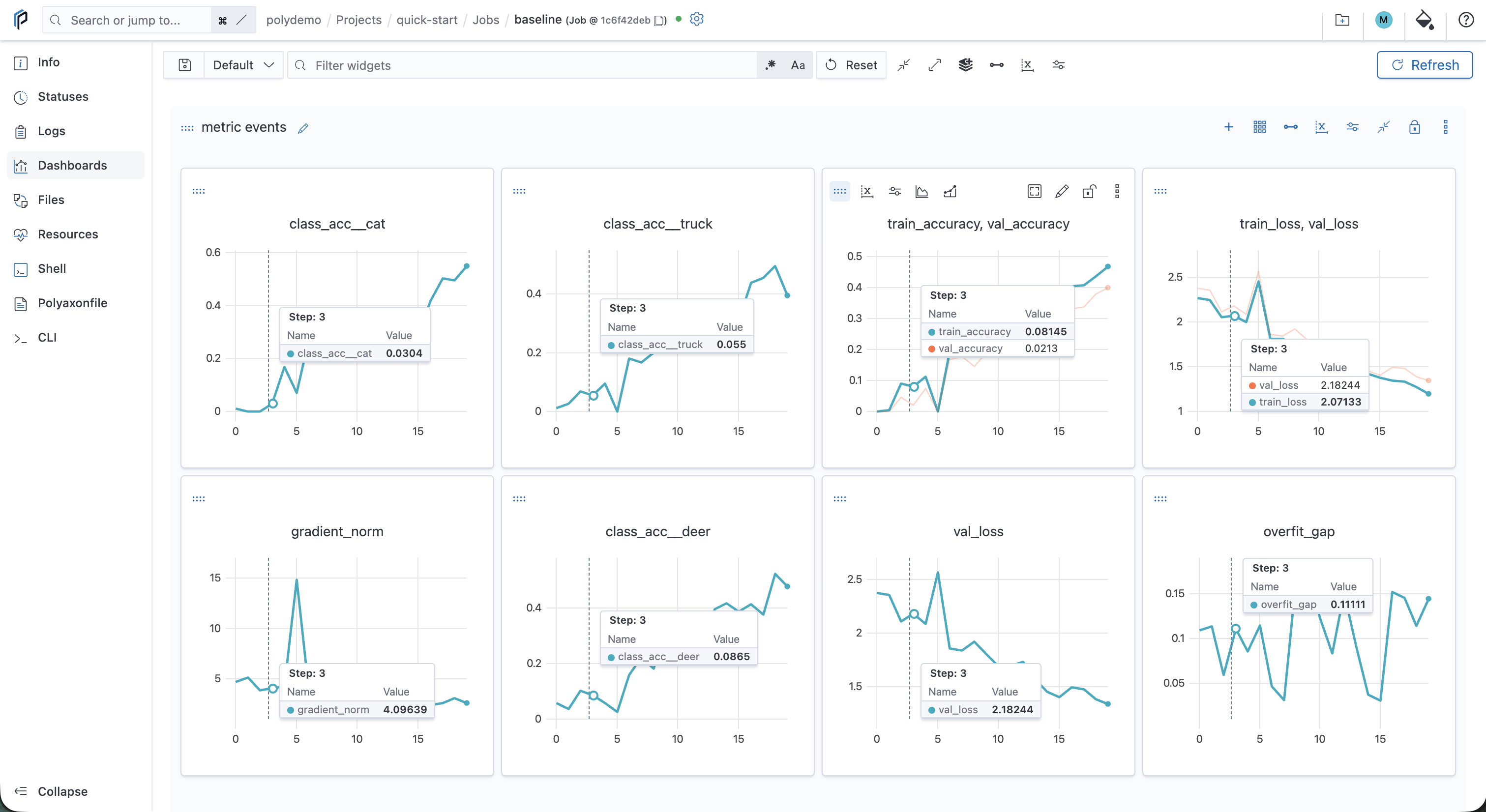
Open Dashboards to inspect the metric history across all 20 epochs.

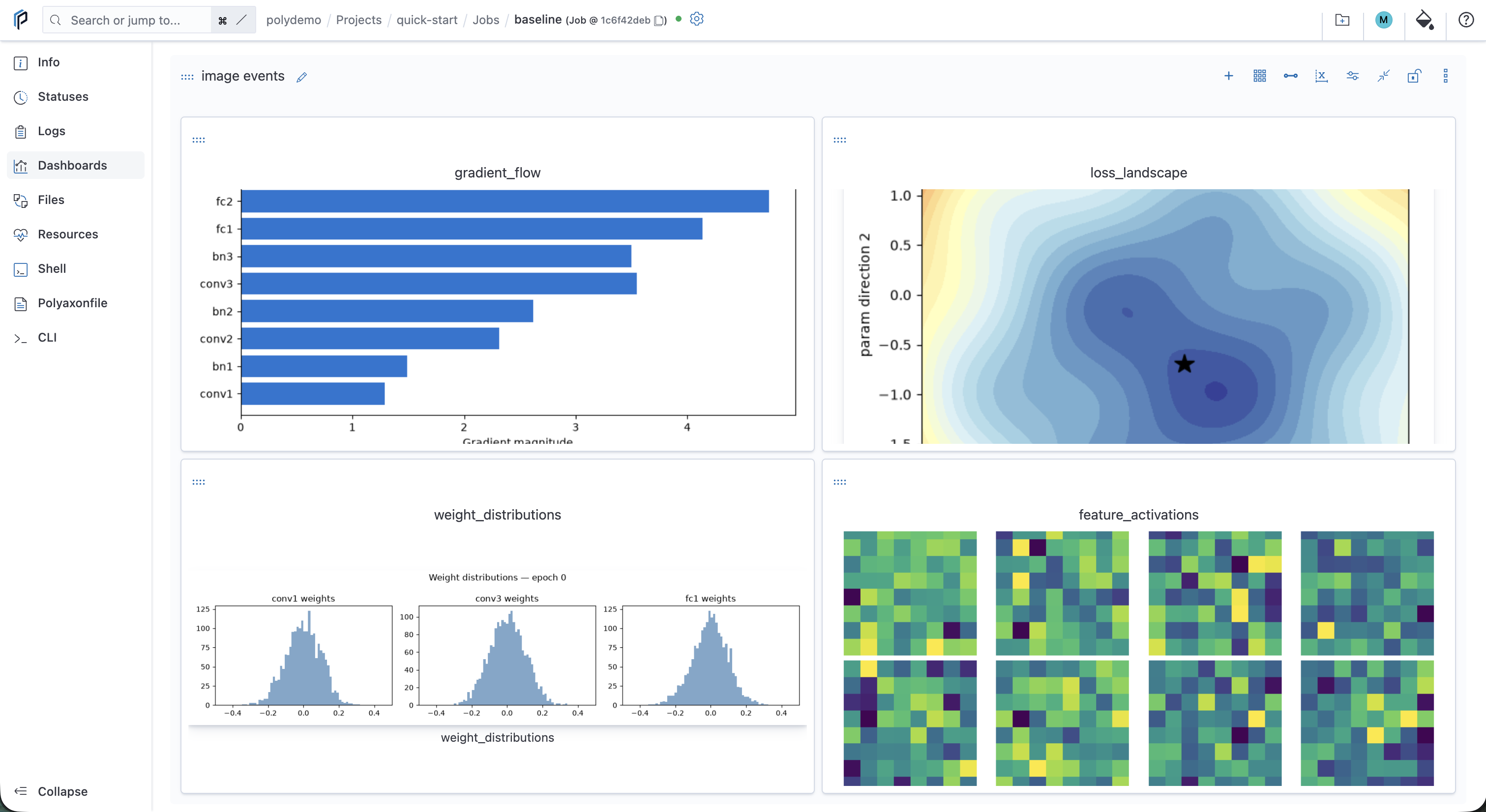
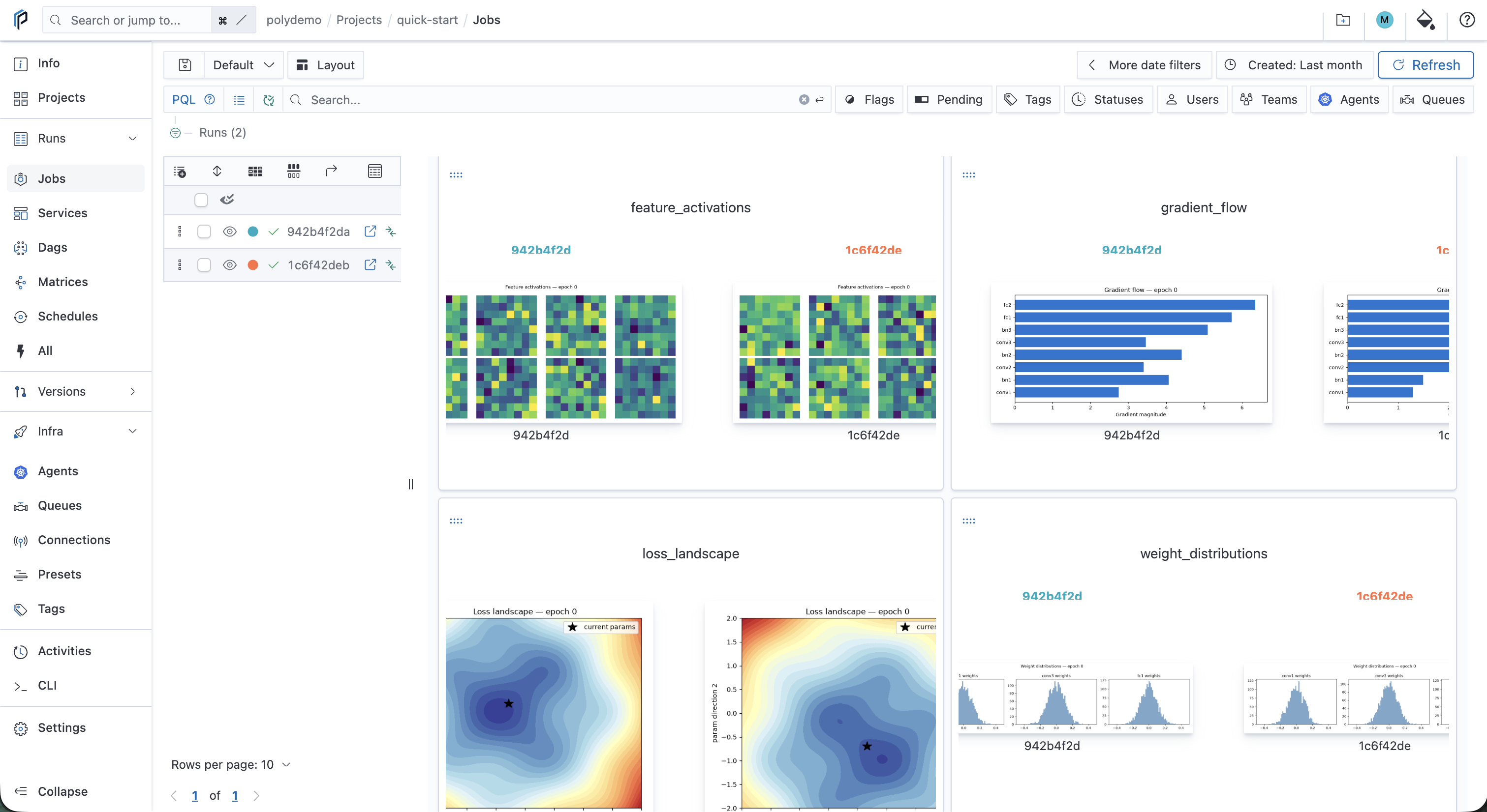
The same dashboard also renders the image events produced by the simulator, including gradient flow, weight distributions, feature activations, and the loss landscape.

Compare two local runs

Run the same simulation with a higher learning rate:

python3 simulate_dl_experiment.py \
  --project=quick-start \
  --run-name=faster-learning-rate \
  --epochs=20 \
  --seed=42 \
  --batch-size=64 \
  --learning-rate=0.003

Both runs execute on your machine with seed 42, 20 epochs, batch size 64, and the simulator defaults for the remaining inputs. The only changed input is the learning rate.

The second run converges faster and finishes with higher validation accuracy, so the effect of the learning-rate change is visible rather than buried in random variation.

Return to the project's runs table, select baseline and faster-learning-rate, then open the comparison view. See Compare runs for the available tables and charts.

The runs table keeps their metadata and results side by side.

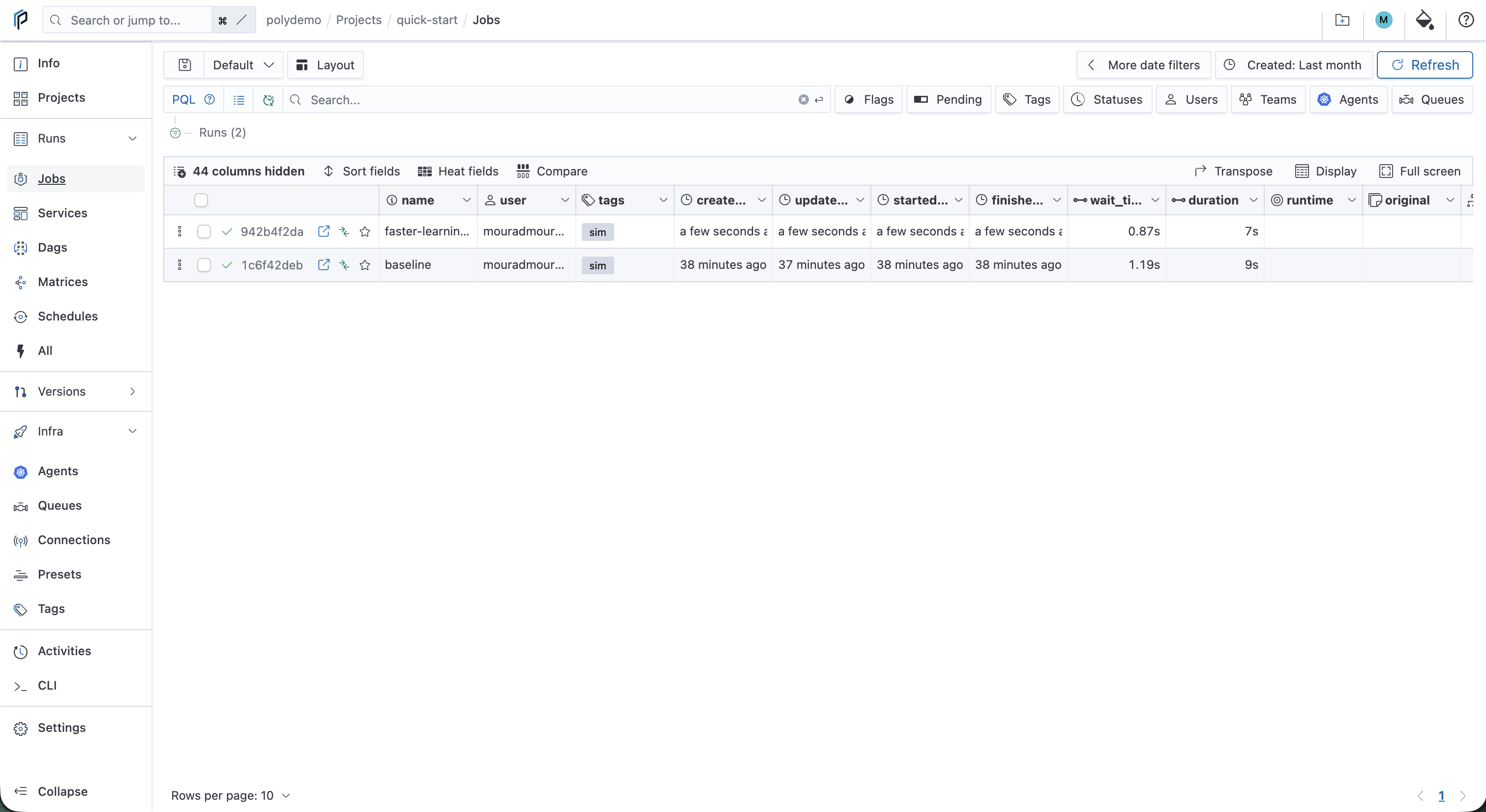
Enable heat fields to make differences in their final outputs easier to scan.

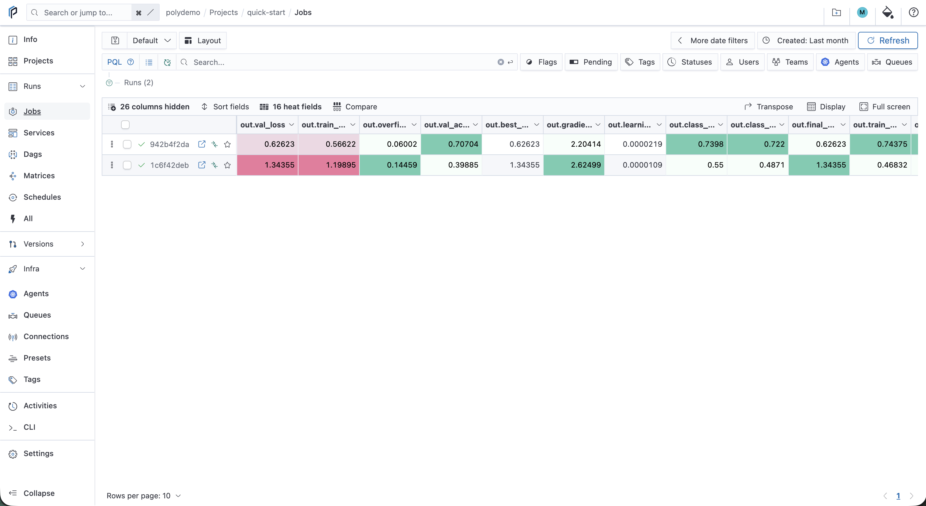
The comparison dashboard overlays their metric histories.

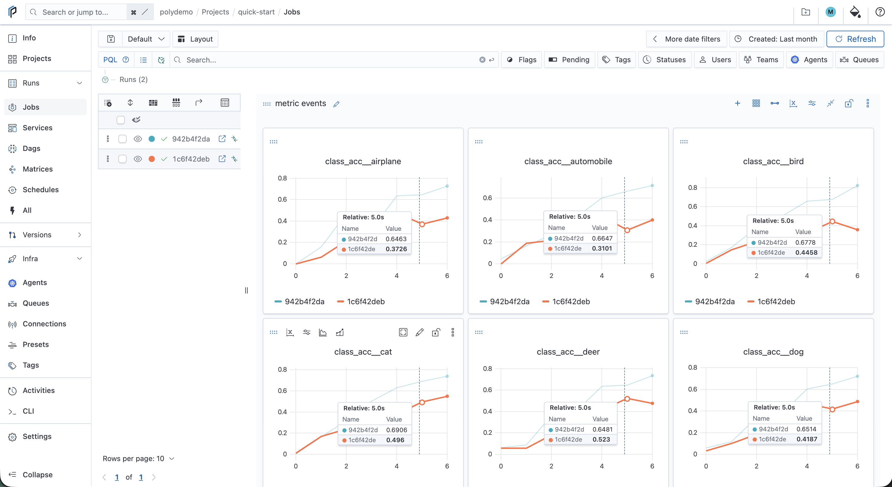
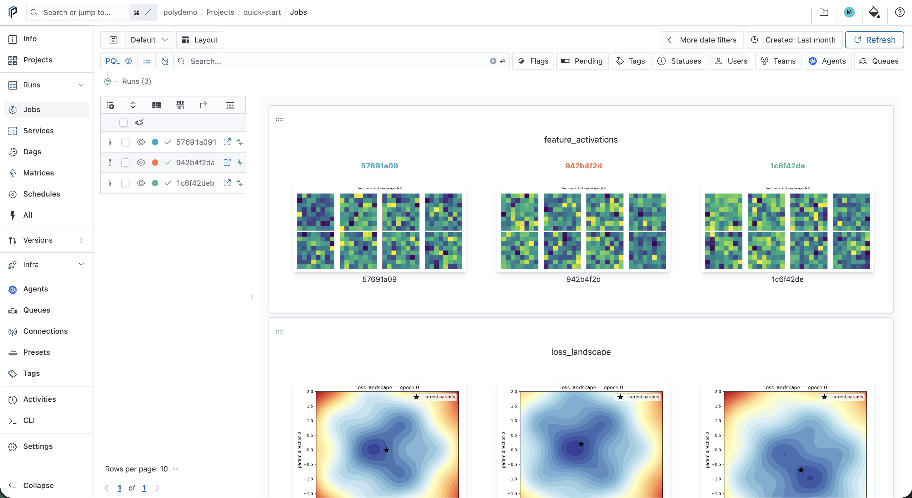
Image comparison places the corresponding visual events from both runs next to each other.

Run the simulator on your cluster

Run a third configuration through the Polyaxon Agent:

polyaxon run \
  -p quick-start \
  --name=managed-faster-learning-rate \
  --tags=sim \
  --url=https://raw.githubusercontent.com/polyaxon/polyaxon-quick-start/master/tracking/simulate.yaml \
  -P epochs=20 \
  -P seed=17 \
  -P batch_size=32 \
  -P learning_rate=0.006 \
  -l

The CLI creates the managed run and prints its dashboard URL. The -l flag then streams its logs.

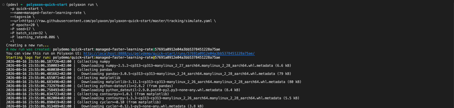
The Agent schedules the simulator's container as a Kubernetes job. You can inspect the same logs in the run view. See the run command reference for more details.

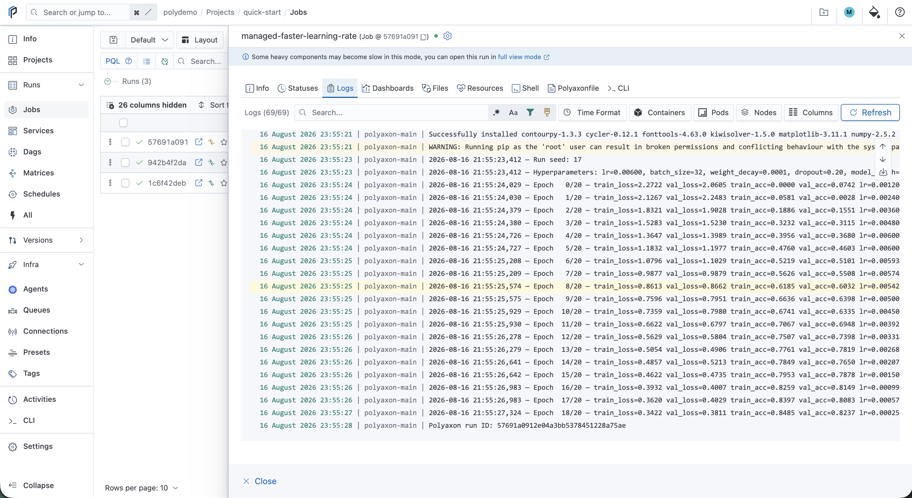
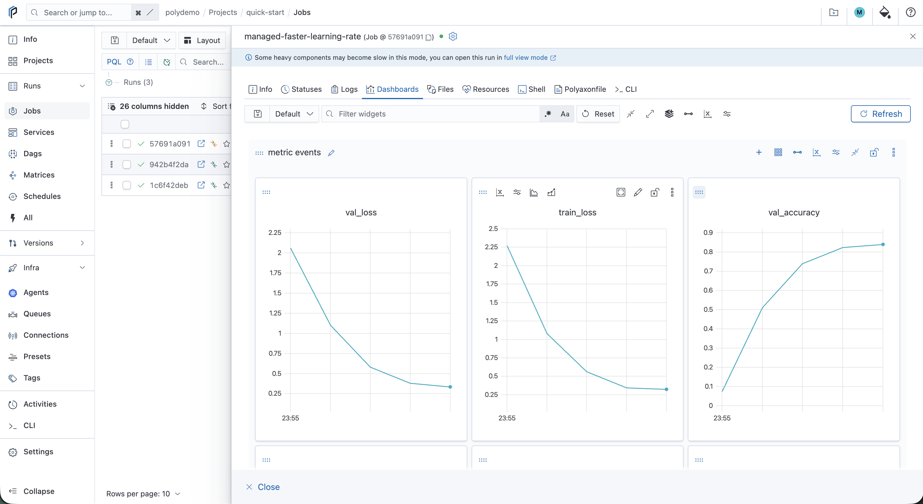
The managed run records the same event types as the local runs.

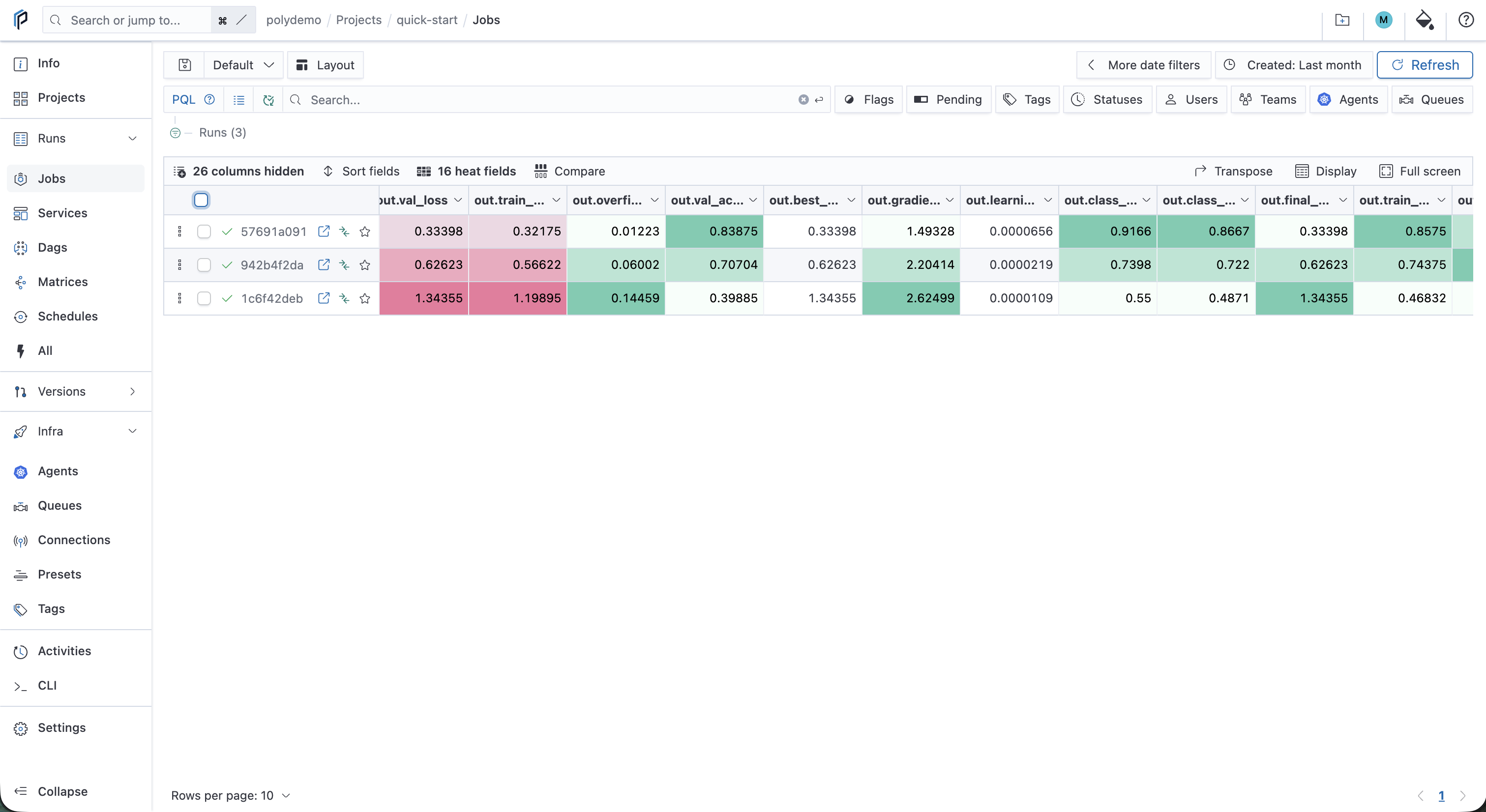
Compare all three runs

Return to the runs table and compare baseline, faster-learning-rate, and managed-faster-learning-rate.

The managed run uses the same simulator with a third set of inputs: seed 17, batch size 32, and learning rate 0.006. This comparison is not a local-versus-cluster performance test. It shows how Polyaxon keeps results from different configurations and execution environments in one project.

Heat fields summarize the three sets of final outputs.

Metric charts show how the three training simulations evolved.

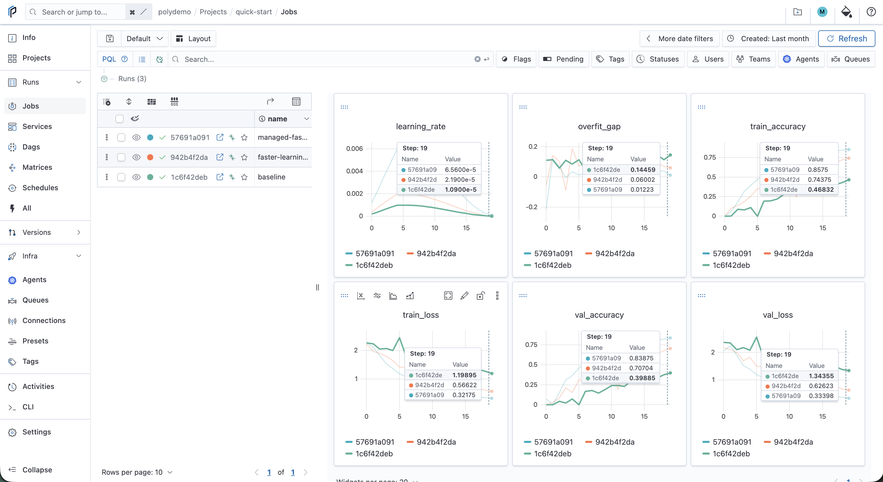
Image comparison applies the same side-by-side view to image events.

What you verified

The baseline and faster-learning-rate runs are user-managed: the simulator ran on your machine and sent its events to Polyaxon. The managed-faster-learning-rate run is managed: the Agent scheduled the same simulator in a container as a Kubernetes job.

This verifies your client configuration, project access, tracking calls, Agent and queue, managed execution, dashboards, and comparisons across local and managed runs.

Next: work interactively

Continue to Interactive development to open a reconnectable shell in a managed simulator environment, run sandbox commands, and try SSH access.

After that, train a TensorFlow model and inspect its results with TensorBoard.

For more ways to instrument local code, see the tracking guide.